R Machine Learning Codebook (Part 1)
- Linear Regression
- Used when response variable is ‘numerical’ variable
getwd()## [1] "/Users/jungyulyang/programming/school/r_blog/content/post"library(readr)
#information for data
usedcar2 <- read_csv("data/usedcar2.csv")## Parsed with column specification:
## cols(
## Price = col_double(),
## Odometer = col_double(),
## Color = col_character()
## )usedcar2## # A tibble: 100 x 3
## Price Odometer Color
## <dbl> <dbl> <chr>
## 1 14636 37388 white
## 2 14122 44758 white
## 3 14470 45854 white
## 4 15072 40149 white
## 5 14802 40237 white
## 6 14660 43533 white
## 7 15612 32744 white
## 8 14632 41350 white
## 9 15008 35781 white
## 10 14666 48613 white
## # … with 90 more rowsEncoding categorical variable
usedcar2$Ind1 <- as.numeric(usedcar2$Color == 'white')
usedcar2$Ind2 <- as.numeric(usedcar2$Color == 'silver')
usedcar2
## # A tibble: 100 x 5
## Price Odometer Color Ind1 Ind2
## <dbl> <dbl> <chr> <dbl> <dbl>
## 1 14636 37388 white 1 0
## 2 14122 44758 white 1 0
## 3 14470 45854 white 1 0
## 4 15072 40149 white 1 0
## 5 14802 40237 white 1 0
## 6 14660 43533 white 1 0
## 7 15612 32744 white 1 0
## 8 14632 41350 white 1 0
## 9 15008 35781 white 1 0
## 10 14666 48613 white 1 0
## # … with 90 more rowsRegression Fitting
lm_used <- lm(Price ~ Odometer + Ind1 + Ind2, data=usedcar2)
summary(lm_used)
##
## Call:
## lm(formula = Price ~ Odometer + Ind1 + Ind2, data = usedcar2)
##
## Residuals:
## Min 1Q Median 3Q Max
## -664.58 -193.42 -5.78 197.38 639.46
##
## Coefficients:
## Estimate Std. Error t value Pr(>|t|)
## (Intercept) 1.670e+04 1.843e+02 90.600 < 2e-16 ***
## Odometer -5.554e-02 4.737e-03 -11.724 < 2e-16 ***
## Ind1 9.048e+01 6.817e+01 1.327 0.187551
## Ind2 2.955e+02 7.637e+01 3.869 0.000199 ***
## ---
## Signif. codes: 0 '***' 0.001 '**' 0.01 '*' 0.05 '.' 0.1 ' ' 1
##
## Residual standard error: 284.5 on 96 degrees of freedom
## Multiple R-squared: 0.698, Adjusted R-squared: 0.6886
## F-statistic: 73.97 on 3 and 96 DF, p-value: < 2.2e-16Plot
plot(lm_used,which=2)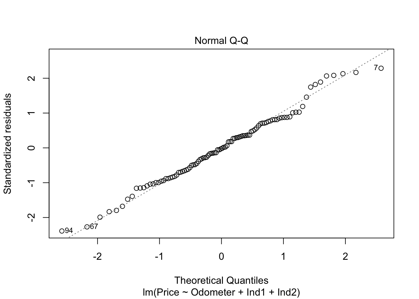
plot(lm_used,which=1)
Things need to check for linear regression 1. Independence 2. Normality 3. Homoscedasticity
X variable Selection
#both = stepwise elimination, backward = backward elimination, forward = forward selection
step_used <- step(lm_used, direction='both')
## Start: AIC=1134.09
## Price ~ Odometer + Ind1 + Ind2
##
## Df Sum of Sq RSS AIC
## - Ind1 1 142641 7915205 1133.9
## <none> 7772564 1134.1
## - Ind2 1 1211971 8984535 1146.6
## - Odometer 1 11129137 18901701 1221.0
##
## Step: AIC=1133.91
## Price ~ Odometer + Ind2
##
## Df Sum of Sq RSS AIC
## <none> 7915205 1133.9
## + Ind1 1 142641 7772564 1134.1
## - Ind2 1 1090245 9005450 1144.8
## - Odometer 1 11056747 18971952 1219.3summary(step_used)##
## Call:
## lm(formula = Price ~ Odometer + Ind2, data = usedcar2)
##
## Residuals:
## Min 1Q Median 3Q Max
## -713.81 -199.46 0.95 183.30 683.18
##
## Coefficients:
## Estimate Std. Error t value Pr(>|t|)
## (Intercept) 1.674e+04 1.826e+02 91.683 < 2e-16 ***
## Odometer -5.533e-02 4.753e-03 -11.640 < 2e-16 ***
## Ind2 2.489e+02 6.809e+01 3.655 0.000417 ***
## ---
## Signif. codes: 0 '***' 0.001 '**' 0.01 '*' 0.05 '.' 0.1 ' ' 1
##
## Residual standard error: 285.7 on 97 degrees of freedom
## Multiple R-squared: 0.6925, Adjusted R-squared: 0.6861
## F-statistic: 109.2 on 2 and 97 DF, p-value: < 2.2e-16Interaction
int_used <- lm(Price ~ Odometer+Ind1+Ind2+Ind1:Odometer+Ind2:Odometer,data=usedcar2)
summary(int_used)
##
## Call:
## lm(formula = Price ~ Odometer + Ind1 + Ind2 + Ind1:Odometer +
## Ind2:Odometer, data = usedcar2)
##
## Residuals:
## Min 1Q Median 3Q Max
## -632.76 -173.28 -7.88 183.62 712.02
##
## Coefficients:
## Estimate Std. Error t value Pr(>|t|)
## (Intercept) 1.708e+04 2.776e+02 61.515 < 2e-16 ***
## Odometer -6.563e-02 7.292e-03 -9.001 2.45e-14 ***
## Ind1 -8.153e+02 4.180e+02 -1.950 0.0541 .
## Ind2 -3.014e+01 4.061e+02 -0.074 0.9410
## Odometer:Ind1 2.399e-02 1.093e-02 2.195 0.0306 *
## Odometer:Ind2 8.445e-03 1.169e-02 0.723 0.4717
## ---
## Signif. codes: 0 '***' 0.001 '**' 0.01 '*' 0.05 '.' 0.1 ' ' 1
##
## Residual standard error: 280.4 on 94 degrees of freedom
## Multiple R-squared: 0.7129, Adjusted R-squared: 0.6976
## F-statistic: 46.68 on 5 and 94 DF, p-value: < 2.2e-16Train Test split
set.seed(1234)
nobs=nrow(usedcar2)
#train:test = 70:30
i = sample(1:nobs, round(nobs*0.7))
train = usedcar2[i,]
test= usedcar2[-i,]
nrow(train);nrow(test)
## [1] 70## [1] 30Prediction and correlation
model = lm(Price ~ Odometer + Ind1 + Ind2, data=train)
pred = predict(model, newdata=test, type = 'response')
pred
## 1 2 3 4 5 6 7 8
## 14676.73 15410.82 14222.10 14947.62 14239.45 14428.65 14392.39 14780.56
## 9 10 11 12 13 14 15 16
## 14637.97 14690.80 14919.48 14576.19 15154.04 15568.29 15190.30 15879.67
## 17 18 19 20 21 22 23 24
## 15118.95 15847.80 15429.82 14124.72 14957.29 14633.57 14539.03 15226.01
## 25 26 27 28 29 30
## 14735.85 14372.92 14047.14 14946.89 14493.71 14658.32cor(test$Price,pred)^2## [1] 0.6832043- Logistic Regression
- Used when response variable is ‘categorical’ variable
directmail <- read_csv("data/directmail.csv")## Parsed with column specification:
## cols(
## RESPOND = col_double(),
## AGE = col_double(),
## BUY18 = col_double(),
## CLIMATE = col_double(),
## FICO = col_double(),
## INCOME = col_double(),
## MARRIED = col_double(),
## OWNHOME = col_double(),
## GENDER = col_character()
## )#remove all na
complete = complete.cases(directmail)
directmail <- directmail[complete,]
directmail## # A tibble: 9,727 x 9
## RESPOND AGE BUY18 CLIMATE FICO INCOME MARRIED OWNHOME GENDER
## <dbl> <dbl> <dbl> <dbl> <dbl> <dbl> <dbl> <dbl> <chr>
## 1 0 71 1 10 719 67 1 0 M
## 2 0 53 0 10 751 72 1 0 M
## 3 0 53 1 10 725 70 1 0 F
## 4 0 45 1 10 684 56 0 0 F
## 5 0 32 0 10 651 66 0 0 F
## 6 0 35 0 10 691 48 0 1 F
## 7 0 43 0 10 694 49 0 1 F
## 8 0 39 0 10 659 64 0 0 M
## 9 0 66 0 10 692 65 0 0 M
## 10 0 52 2 10 705 58 1 1 M
## # … with 9,717 more rowsnobs=nrow(directmail)
#train:test = 70:30
i = sample(1:nobs, round(nobs*0.7))
train = directmail[i,]
test= directmail[-i,]
nrow(train);nrow(test)## [1] 6809## [1] 2918Logistic Fitting
full_model = glm(RESPOND ~ AGE+BUY18+CLIMATE+FICO+INCOME+MARRIED+OWNHOME+GENDER,
                 family='binomial',data=directmail)
summary(full_model)
##
## Call:
## glm(formula = RESPOND ~ AGE + BUY18 + CLIMATE + FICO + INCOME +
## MARRIED + OWNHOME + GENDER, family = "binomial", data = directmail)
##
## Deviance Residuals:
## Min 1Q Median 3Q Max
## -1.1544 -0.4275 -0.3582 -0.2941 2.9353
##
## Coefficients:
## Estimate Std. Error z value Pr(>|z|)
## (Intercept) 2.713421 0.948186 2.862 0.00421 **
## AGE -0.037951 0.004469 -8.491 < 2e-16 ***
## BUY18 0.461354 0.058442 7.894 2.92e-15 ***
## CLIMATE -0.020629 0.006271 -3.289 0.00100 **
## FICO -0.004988 0.001326 -3.760 0.00017 ***
## INCOME -0.001425 0.002499 -0.570 0.56851
## MARRIED 0.534643 0.090075 5.936 2.93e-09 ***
## OWNHOME -0.421534 0.090408 -4.663 3.12e-06 ***
## GENDERM -0.076648 0.079758 -0.961 0.33655
## ---
## Signif. codes: 0 '***' 0.001 '**' 0.01 '*' 0.05 '.' 0.1 ' ' 1
##
## (Dispersion parameter for binomial family taken to be 1)
##
## Null deviance: 5179.6 on 9726 degrees of freedom
## Residual deviance: 4977.5 on 9718 degrees of freedom
## AIC: 4995.5
##
## Number of Fisher Scoring iterations: 5Predict Probability
prob_pred = predict(full_model, newdata=test, type="response")ROC CURVE
library(pROC)## Type 'citation("pROC")' for a citation.##
## Attaching package: 'pROC'## The following objects are masked from 'package:stats':
##
## cov, smooth, varroccurve <- roc(test$RESPOND ~ prob_pred)## Setting levels: control = 0, case = 1## Setting direction: controls < casesplot(roccurve,col="red",print.auc=TRUE, print.auc.adj=c(1,-7),auc.polygon=TRUE)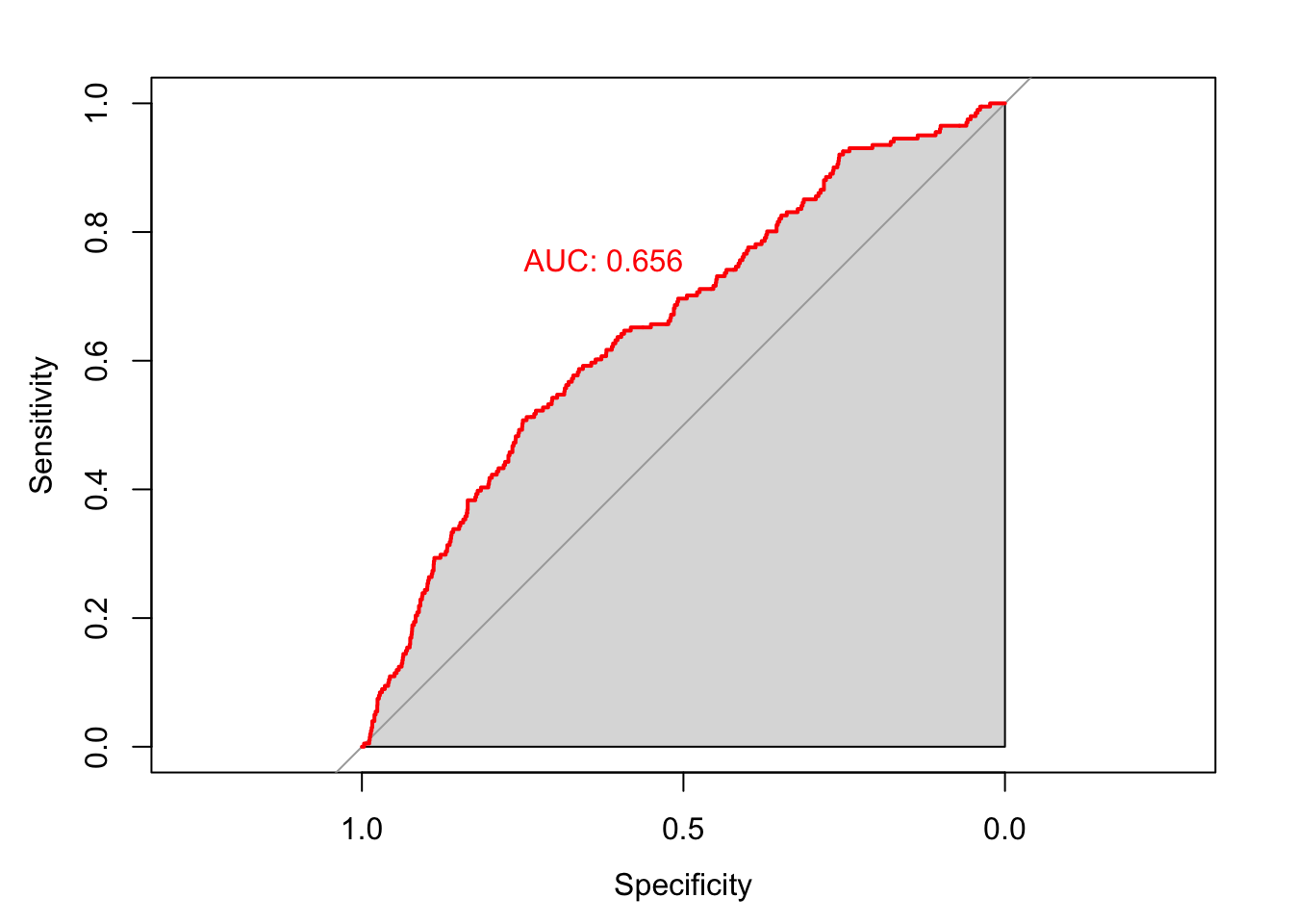
- Decision Trees
- Used regardless of the type of response variable
library(readr)
titanic <- read_csv("data/titanic.csv")
## Parsed with column specification:
## cols(
## Class = col_character(),
## Age = col_character(),
## Sex = col_character(),
## Survived = col_character()
## )titanic## # A tibble: 2,201 x 4
## Class Age Sex Survived
## <chr> <chr> <chr> <chr>
## 1 First Adult Male Yes
## 2 First Adult Male Yes
## 3 First Adult Male Yes
## 4 First Adult Male Yes
## 5 First Adult Male Yes
## 6 First Adult Male Yes
## 7 First Adult Male Yes
## 8 First Adult Male Yes
## 9 First Adult Male Yes
## 10 First Adult Male Yes
## # … with 2,191 more rowsTree Fitting
#class represents tree where anova represents regression tree
library(rpart)
library(rpart.plot)
D_tree <- rpart(Survived ~ Class+Sex+Age, data=titanic, method='class')
print(D_tree)
## n= 2201
##
## node), split, n, loss, yval, (yprob)
## * denotes terminal node
##
## 1) root 2201 711 No (0.6769650 0.3230350)
## 2) Sex=Male 1731 367 No (0.7879838 0.2120162)
## 4) Age=Adult 1667 338 No (0.7972406 0.2027594) *
## 5) Age=Child 64 29 No (0.5468750 0.4531250)
## 10) Class=Third 48 13 No (0.7291667 0.2708333) *
## 11) Class=First,Second 16 0 Yes (0.0000000 1.0000000) *
## 3) Sex=Female 470 126 Yes (0.2680851 0.7319149)
## 6) Class=Third 196 90 No (0.5408163 0.4591837) *
## 7) Class=Crew,First,Second 274 20 Yes (0.0729927 0.9270073) *prp(D_tree, type=4, extra=2, digits=3)
More parameters to control
#xval means cross validation, whether to prun or not
my.control <- rpart.control(xval=10,cp=0.001,minsplit=3)
tree <- rpart(Survived ~ Class+Sex+Age, data=titanic, method='class', control = my.control)
plot(tree, uniform=T, compress = T, margin=0.05)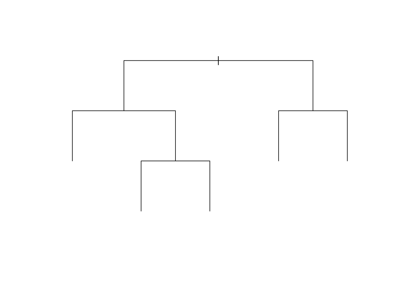
printcp(tree)##
## Classification tree:
## rpart(formula = Survived ~ Class + Sex + Age, data = titanic,
## method = "class", control = my.control)
##
## Variables actually used in tree construction:
## [1] Age Class Sex
##
## Root node error: 711/2201 = 0.32303
##
## n= 2201
##
## CP nsplit rel error xerror xstd
## 1 0.306610 0 1.00000 1.00000 0.030857
## 2 0.022504 1 0.69339 0.69339 0.027510
## 3 0.011252 2 0.67089 0.69620 0.027549
## 4 0.001000 4 0.64838 0.64838 0.026850