- Neural Network
- used regardless of response variable, but intended to predict
library(readr)
directmail <- read_csv("data/directmail.csv")
## Parsed with column specification:
## cols(
## RESPOND = col_double(),
## AGE = col_double(),
## BUY18 = col_double(),
## CLIMATE = col_double(),
## FICO = col_double(),
## INCOME = col_double(),
## MARRIED = col_double(),
## OWNHOME = col_double(),
## GENDER = col_character()
## )#remove all na
complete = complete.cases(directmail)
directmail <- directmail[complete,]
directmail## # A tibble: 9,727 x 9
## RESPOND AGE BUY18 CLIMATE FICO INCOME MARRIED OWNHOME GENDER
## <dbl> <dbl> <dbl> <dbl> <dbl> <dbl> <dbl> <dbl> <chr>
## 1 0 71 1 10 719 67 1 0 M
## 2 0 53 0 10 751 72 1 0 M
## 3 0 53 1 10 725 70 1 0 F
## 4 0 45 1 10 684 56 0 0 F
## 5 0 32 0 10 651 66 0 0 F
## 6 0 35 0 10 691 48 0 1 F
## 7 0 43 0 10 694 49 0 1 F
## 8 0 39 0 10 659 64 0 0 M
## 9 0 66 0 10 692 65 0 0 M
## 10 0 52 2 10 705 58 1 1 M
## # … with 9,717 more rowsnobs=nrow(directmail)
#normalization
nor = function(x) {x-min(x)/(max(x)-min(x))}
directmail$AGE <- nor(directmail$AGE)
directmail$CLIMATE <- nor(directmail$CLIMATE)
directmail$FICO <- nor(directmail$FICO)
directmail$INCOME <- nor(directmail$INCOME)
directmail$GENDER <- as.numeric(directmail$GENDER == "F")#split
set.seed(1234)
i = sample(1:nobs, round(nobs*0.7))
train = directmail[i,]
test = directmail[-i,]
nrow(train);nrow(test)## [1] 6809## [1] 2918Neural Network Fitting
#stepmax : iteration, threshold: error variation, act.fact : function
library(neuralnet)
nn <- neuralnet(RESPOND ~ AGE+BUY18+CLIMATE+FICO+INCOME+MARRIED+OWNHOME+GENDER,
                data=train, hidden=3, step = 1e+05, threshold = 0.01,
                act.fct = 'logistic', linear.output=F)
plot(nn)
Prediction
pred <- compute(nn, covariate=test[,-1])- Ensemble
- Bagging
german = read.table("data/germandata.txt",header=T)
german$numcredits = factor(german$numcredits)
german$residence = factor(german$residence)
german$residpeople = factor(german$residpeople)
summary(german)
## check duration history purpose credit savings
## A11:274 Min. : 4.0 A30: 40 A43 :280 Min. : 250 A61:603
## A12:269 1st Qu.:12.0 A31: 49 A40 :234 1st Qu.: 1366 A62:103
## A13: 63 Median :18.0 A32:530 A42 :181 Median : 2320 A63: 63
## A14:394 Mean :20.9 A33: 88 A41 :103 Mean : 3271 A64: 48
## 3rd Qu.:24.0 A34:293 A49 : 97 3rd Qu.: 3972 A65:183
## Max. :72.0 A46 : 50 Max. :18424
## (Other): 55
## employment installment personal debtors residence property
## A71: 62 Min. :1.000 A91: 50 A101:907 1:130 A121:282
## A72:172 1st Qu.:2.000 A92:310 A102: 41 2:308 A122:232
## A73:339 Median :3.000 A93:548 A103: 52 3:149 A123:332
## A74:174 Mean :2.973 A94: 92 4:413 A124:154
## A75:253 3rd Qu.:4.000
## Max. :4.000
##
## age others housing numcredits job residpeople
## Min. :19.00 A141:139 A151:179 1:633 A171: 22 1:845
## 1st Qu.:27.00 A142: 47 A152:713 2:333 A172:200 2:155
## Median :33.00 A143:814 A153:108 3: 28 A173:630
## Mean :35.55 4: 6 A174:148
## 3rd Qu.:42.00
## Max. :75.00
##
## telephone foreign y
## A191:596 A201:963 bad :300
## A192:404 A202: 37 good:700
##
##
##
##
## Bagging Fitting
library(rpart)
library(adabag)
## Loading required package: caret## Loading required package: lattice## Loading required package: ggplot2## Loading required package: foreach## Loading required package: doParallel## Loading required package: iterators## Loading required package: parallelset.seed(1234)
my.control <- rpart.control(xval=0, cp=0, minsplit=5, maxdepth=10)
bag.german <- bagging(y ~ . , data=german, mfinal=50, control=my.control)
summary(bag.german)## Length Class Mode
## formula 3 formula call
## trees 50 -none- list
## votes 2000 -none- numeric
## prob 2000 -none- numeric
## class 1000 -none- character
## samples 50000 -none- numeric
## importance 20 -none- numeric
## terms 3 terms call
## call 5 -none- callVariable Importance
print(bag.german$importance)## age check credit debtors duration employment
## 7.1522348 16.8217396 12.5679179 2.2181683 11.0256049 5.9617574
## foreign history housing installment job numcredits
## 0.0000000 6.8068853 1.1459084 2.2181232 2.5859388 0.8272318
## others personal property purpose residence residpeople
## 2.3088330 2.4362463 4.1130547 11.4096016 3.8042727 0.5134954
## savings telephone
## 5.4490034 0.6339825importanceplot(bag.german)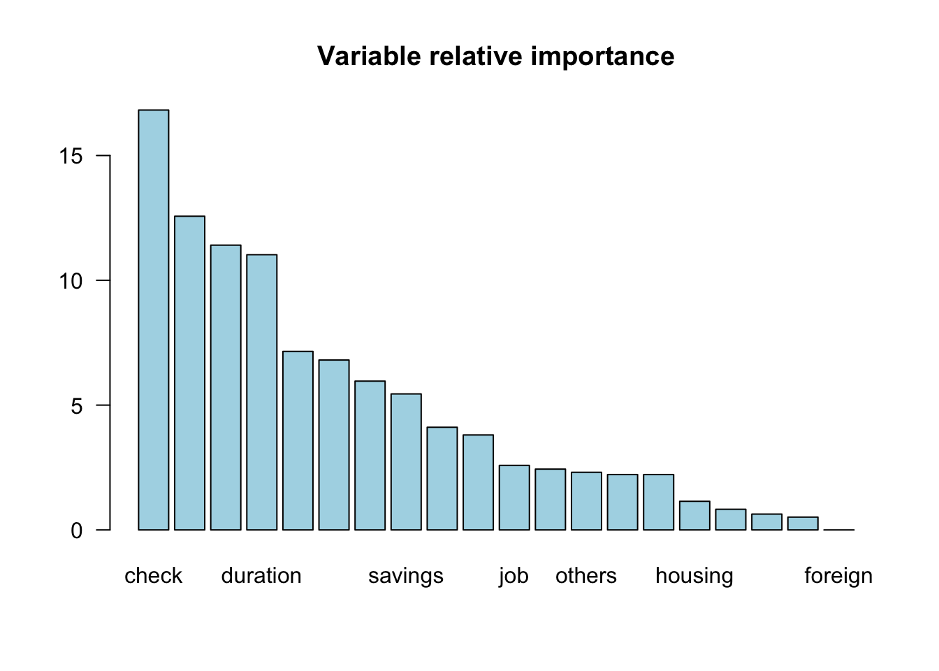
Prediction
pred.bag.german <- predict.bagging(bag.german, newdata=german)
head(pred.bag.german$prob,10)
## [,1] [,2]
## [1,] 0.02 0.98
## [2,] 0.90 0.10
## [3,] 0.04 0.96
## [4,] 0.34 0.66
## [5,] 0.72 0.28
## [6,] 0.12 0.88
## [7,] 0.00 1.00
## [8,] 0.16 0.84
## [9,] 0.00 1.00
## [10,] 0.88 0.12Confusion matrix
print(pred.bag.german$confusion)## Observed Class
## Predicted Class bad good
## bad 272 3
## good 28 697- Boosting
my.control <- rpart.control(xval=0,cp=0, maxdepth=1)
boo.german <- boosting(y ~ . , data=german, boos=T, mfinal=100, control=my.control)
summary(boo.german)
## Length Class Mode
## formula 3 formula call
## trees 100 -none- list
## weights 100 -none- numeric
## votes 2000 -none- numeric
## prob 2000 -none- numeric
## class 1000 -none- character
## importance 20 -none- numeric
## terms 3 terms call
## call 6 -none- callevol.german = errorevol(boo.german, newdata=german)
plot.errorevol(evol.german)
- RandomForest
- randomforest chooses some variable randomly instead of choosing all variables
Random Forest Fitting
library(randomForest)## randomForest 4.6-14## Type rfNews() to see new features/changes/bug fixes.##
## Attaching package: 'randomForest'## The following object is masked from 'package:ggplot2':
##
## marginrf.german <- randomForest(y~., data=german, ntree= 100, mtry=5, importance=T, na.action=na.omit)
summary(rf.german)## Length Class Mode
## call 7 -none- call
## type 1 -none- character
## predicted 1000 factor numeric
## err.rate 300 -none- numeric
## confusion 6 -none- numeric
## votes 2000 matrix numeric
## oob.times 1000 -none- numeric
## classes 2 -none- character
## importance 80 -none- numeric
## importanceSD 60 -none- numeric
## localImportance 0 -none- NULL
## proximity 0 -none- NULL
## ntree 1 -none- numeric
## mtry 1 -none- numeric
## forest 14 -none- list
## y 1000 factor numeric
## test 0 -none- NULL
## inbag 0 -none- NULL
## terms 3 terms callVariable Importance
importance(rf.german,type=1)## MeanDecreaseAccuracy
## check 16.4639651
## duration 5.6544313
## history 6.5430882
## purpose 2.5991136
## credit 5.6596124
## savings 4.6071442
## employment 3.5484219
## installment 1.8982220
## personal 2.6265059
## debtors 2.8674523
## residence 0.7142969
## property 3.9839084
## age 2.9140090
## others 4.6528737
## housing 0.9793288
## numcredits 0.8780246
## job 0.2996086
## residpeople 0.6849617
## telephone 2.1266027
## foreign 1.5613566Prediction
pred.rf.german <- predict(rf.german, newdata=german)
head(pred.rf.german,10)
## 1 2 3 4 5 6 7 8 9 10
## good bad good good bad good good good good bad
## Levels: bad goodConfusion matrix
tab = table(german$y,pred.rf.german , dnn = c("Actual","Predicted"))
print(tab)
## Predicted
## Actual bad good
## bad 300 0
## good 0 700